In one paragraph
Give gemma-2-2b a Python function that accumulates into a local variable,
and cut the prompt off right after return. The model predicts
result, the accumulator it bound four lines earlier, with
95.3% probability. I used
circuit-tracer
to build an attribution graph over that prediction. The answer is not a
frequency prior over common variable names. A specific mid-layer feature fires on the
result tokens, and a band of late-layer features on return
adds to the same logit.
One graph cannot say whether that feature tracks the variable being bound or
simply the name result. In this prompt they coincide.
Control prompts that move the binding around separate the two,
and the answer is the name. Each variable name has its own pathway, and the
pathways are orthogonal. The nodes sitting on result drive the
result logit and essentially nothing else. The nodes sitting on a
second name, ans, drive ans and essentially nothing
else. Binding does not switch a pathway on or off. It sets how much drive
that name accumulates, and the model takes the winner at the logit layer.
Three things then hold this up. Across five graphs no pathway pushes the rival logit
by more than 2.0 while pushing its own by 17 to 39. The effect
is not about the word result: 18 accumulator
names behave the same way over four prompt shapes, including runnable Python.
And it is causal: scale the winning name's feature down and
the probabilities cross over, so the model returns the other variable.
Before the graph, there is a cheaper question: where the model
looks from return. The answer is the same in every prompt. The heads
that carry the names attend to the assignment line and the loop line, and what changes
between prompts is the name that happens to sit there.
The task
The prompt is a complete, unambiguous function whose body binds one local variable. Everything the model needs to answer correctly is in scope. Nothing in the surrounding text hints at the name. This is the first of four prompts, P1. The other three are controls (P2–P4) that move the binding around, and the interpretation ultimately rests on them.
P1 · return-variable. result is bound twice.
def calculate_total(prices):
    result = 0
    for price in prices:
        result = result + price
    return
That is 31 tokens including <bos>. The two writes to
result land at positions 10 and 23.
The final return is position 30, and that is where the
next-token prediction is made.
What the model predicts
| Rank | Token | Probability |
|---|---|---|
| 1 | result | 95.31% |
| 2 | ( | 1.06% |
| 3 | round | 0.59% |
| 4 | ( | 0.52% |
| 5 | int | 0.28% |
| 6 | price | 0.26% |
Note the sixth entry. price, the loop variable, is the plausible
wrong answer. A model that merely knew "a variable name goes here" could easily
produce it. It gets 0.26%. Whatever the model is doing, it distinguishes the
accumulator from the iteration variable.
Where the return position looks
The attribution graph below says what is moved toward each logit. It does not
say where the model looks to fetch it. That is the QK side of each attention
head, and it can be read straight off the attention pattern at the return
position: one forward pass per prompt, no transcoders. The figure takes the ten heads
that put the most attention mass on the two candidate names in P4, drops the BOS column
(an attention sink that soaks up about 0.4 of the raw mass on average), renormalises the
rest, and shows the same ten rows for all four prompts on one colour scale. Blue boxes
mark the result tokens, red boxes the ans tokens.
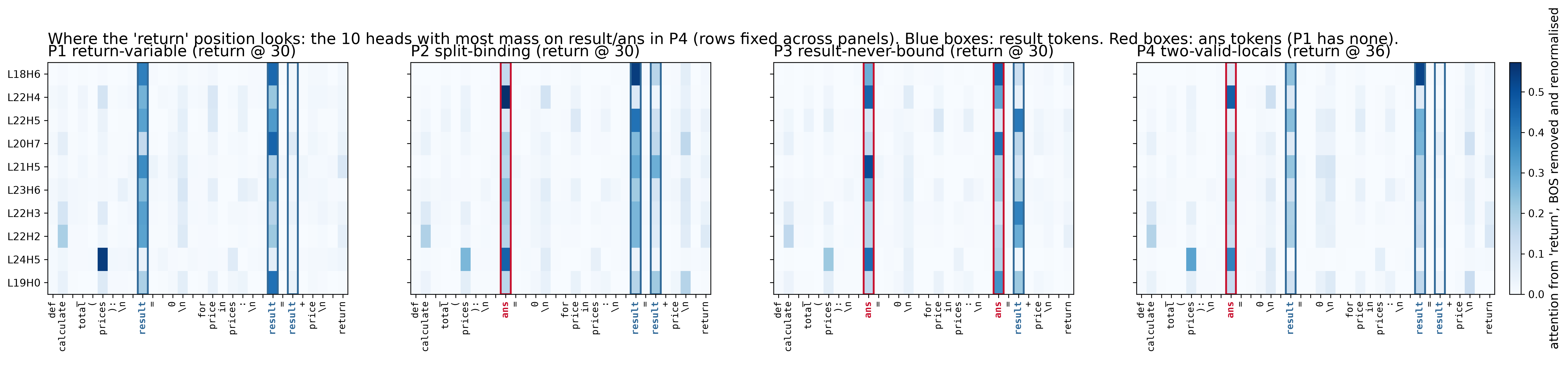
return, BOS removed and renormalised. Rows are the ten
heads with most mass on result / ans in P4, fixed across
panels. P1 has no ans, so it carries blue boxes only. Same figure as
the poster's WHERE band; generated by attention_at_return.py and
replotted from the committed .npy matrices.
Three things to read off it. First, on P1 there is only one name on the page and the
heads put their mass on it: L18H6 places 0.87 of its renormalised attention on the
result tokens. Second, counted by name, P2 and P3 look different.
L18H6 gives result 0.71 of its mass in P2 and 0.13 in P3, and
ans the reverse. Third, counted by position, the same head looks at
the same places in both: the assignment on line 2 and the accumulation inside the loop.
Over the ten heads, the cosine between a head's P2 row and its P3 row has median 0.86;
over all 208 heads it is 0.99. The heads attend to the structure of the function, and
the name that happens to sit at those positions is what changes.
Two of these heads, L18H6 and L21H5, are among the model's strongest induction heads:
0.79 and 0.67 on repeated random token sequences, with a previous-token score under
0.04. That is the 2022 mechanism, [A][B]…[A] → [B], applied to a
variable name that appeared earlier in the function.
Attention says where, not what. High weight on a token does not by itself mean that token's content is what moved the logit; Jain and Wallace (2019) make the point at length. The heatmap never stands alone here. The graph says what is moved, and the intervention says whether it matters.
Numbers: attention_return_summary.txt (masses, cosines, the branch decision)
and head_scores.csv (all 208 heads) in the experiment outputs.
The circuit
result logit. That is the only logit target in this graph, since the top
prediction cleared the 0.95 coverage threshold on its own. The full graph (1,460
nodes and 56,975 edges) is explorable interactively.
Largest direct effects on the result logit
| Node | Direct effect | Position | What it is |
|---|---|---|---|
| 18_4769_10 | +5.34 | 10 | Layer-18 feature 4769 on the first result, where it is bound (activation 103) |
| 24_15424_30 | −5.09 | 30 | Layer-24 feature on return, the main suppressor |
| 18_4769_23 | +2.73 | 23 | The same feature 4769, on the accumulation line (activation 44) |
| E_10 | +2.56 | 10 | Raw token embedding of the first result |
| E_23 | +2.20 | 23 | Raw token embedding of the second result |
| 24_12518_30 | +0.89 | 30 | Late-layer feature on return |
| 18_4769_14 | +0.78 | 14 | Feature 4769 again, on the newline closing result = 0 |
| 21_5255_30 | +0.61 | 30 | Late-layer feature on return |
| 25_4717_30 | +0.51 | 30 | Late-layer feature on return (activation 252) |
Three things stand out.
One feature carries most of the positive effect, and it fires only on
result. Feature 18_4769 is the single largest
positive contributor. It appears three times in the top nine: at both writes to
result and at the newline that closes the first one. It never fires on
price or prices. Two readings fit this one graph equally
well: a feature for "the local variable being assigned here", or a feature for the
name result. The controls decide between
them. 18_4769 is tied to the name, and it stays silent through a
perfectly good binding of a different name.
The raw embeddings contribute directly. E_10 and
E_23, the plain token embeddings of the two result
occurrences, contribute +2.56 and +2.20 without passing through any feature. That is
a copy path straight from the input. In the controls this path
carries a large share of each name's total, and it is name-specific in the same way
the features are.
The largest single effect is negative. 24_15424_30
pushes the result logit down by 5.09, almost exactly
cancelling the top promoter. The prediction survives because the promoting evidence
is distributed across many nodes, not because any one of them overwhelms the
suppressor. The controls settle what this feature is:
result's own dedicated suppressor. It fires
against result just as hard when result is
losing. When the accumulator is a different name, a different
layer-24 feature takes its place.
Most influential nodes overall
Direct effect measures one row of the adjacency matrix. Ranking instead by total influence (direct and indirect, the score the pruner uses) puts the structural tokens first:
| Rank | Node | Token | Kind |
|---|---|---|---|
| 1 | E_1 | def | embedding |
| 2 | E_0 | <bos> | embedding |
| 3 | E_10 | result | embedding |
| 4 | E_2 | calculate | embedding |
| 5 | 18_4769_10 | result | feature |
| 6 | E_6 | prices | embedding |
| 7 | E_4 | total | embedding |
| 8 | 24_15424_30 | return | feature |
def and <bos> leading this ranking is expected. They
gate the whole "this is a Python function body" computation, so almost everything
routes through them. The informative entry is 18_4769_10 at rank 5.
The identifier feature is influential on both measures, which is what separates it
from nodes that merely sit on a busy path.
The controls
One prompt is not enough to interpret. In the function above, the
name result and the variable that gets bound are the same thing. A
feature that fires on result could be tracking either. The controls
below pull the two apart, and they come down on the side of the name.
Each control keeps the function, the loop and the cut point identical, and changes only which name is bound where. Two of them are deliberately invalid Python because a name is read before it is ever assigned. Making binding and mere occurrence disagree is the only way to tell which one the model follows. The third is ordinary runnable code. It is the one to check first if the invalid ones bother you.
P2 · split-binding. ans is bound; result is
accumulated into but never initialised. Invalid Python.
def calculate_total(prices):
    ans = 0
    for price in prices:
        result = result + price
    return
P3 · result-never-bound. ans is bound twice;
result only ever appears on a right-hand side. Invalid Python.
def calculate_total(prices):
    ans = 0
    for price in prices:
        ans = result + price
    return
P4 · two-valid-locals. Both names are bound, and only result
is accumulated into. This one runs.
def calculate_total(prices):
    ans = 0
    result = 0
    for price in prices:
        result = result + price
    return
How a prompt is scored
The same conventions as the two companion pages, with one difference. There are no pairs and no verdicts here. The question is which name the model picks and by how much, rather than whether it is right. Four layers, each with its own measurement:
-
Behaviour (P1–P4). One forward pass per prompt, cut
immediately after
return. The model sees the function and nothing else: no primer, no examples. From the softmax at that position the table reports P(result) and P(ans), the two candidate names. Each is a single token with its leading space. The answer is the top-1 over the whole vocabulary, not just the two candidates. That is why(,roundandpriceappear in the P1 top-k above: the names compete inside a real next-token distribution. -
Name sweep (18 names × 4 shapes). Same forward pass, with
the accumulator replaced by each of 18 single-token names and
anskept as the distractor. A case isokif the top-1 token is the name the binding account predicts (the accumulator, or the distractor undernever-bound). An exact tie is counted aMISS, for the same reason the companion pages score ties as neither: argmax would break it toward whichever candidate is listed first. The margin, P(predicted) − P(other), is reported, not thresholded. - Attribution (per-logit aggregates). A magnitude, not a verdict. For each graph, every node sitting on a name's token positions is summed by its direct effect on one named logit. The graph carries every logit whose cumulative probability is needed to reach 0.95, so P2–P4 have two or three targets and P1 has one. A node's effect on the top logit and on the other logit are two different numbers, and both are reported.
- Intervention. The same forward pass with one feature clamped to a fraction of its value at every position it fires, then the same two probabilities read off. The harness reports its unmodified baseline first. It must reproduce the behaviour probe (95.31 / 69.14 / 6.45%) before any intervention number is believed.
| P | Prompt | Binding | Runs? | result | ans |
|---|---|---|---|---|---|
| P1 | return-variable | result bound twice | yes | 95.70% | 0.00% |
| P2 | split-binding | ans bound at line 2, result in the loop | no | 68.75% | 25.20% |
| P3 | result-never-bound | ans bound twice, result read only | no | 6.45% | 89.06% |
| P4 | two-valid-locals | both bound, only result grows | yes | 82.42% | 11.18% |
Binding clearly matters to the behaviour: move it and the answer moves with it, from 95.7% down to 6.5%. The question is how, and for that the graphs have to be read carefully.
Every number needs a named logit
A direct effect is meaningless until you say which logit it is measured against. The first prompt's graph has a single logit target, so there is nothing there to get wrong. The controls each carry several, because both names clear the coverage threshold. A node's effect on the top logit can be near zero while its effect on the other logit is large. Every number below names its target.
For each graph, take every node sitting on a name's tokens and sum its direct effect
on each logit separately. P2, P3 and P4 each have two candidate names. Two more
graphs, split-total and total-never-bound, repeat P2 and P3
with total as the accumulator. They check that nothing here is about the
word result:
| Graph | Returned | → own logit | → other | Loser | → own logit | → other |
|---|---|---|---|---|---|---|
| P2 split-binding | result |
+26.963 | +1.389 | ans | +20.268 | +0.049 |
| P3 result-never-bound | ans |
+26.957 | +0.700 | result | +17.027 | +0.921 |
| P4 two-valid-locals | result |
+37.301 | +1.996 | ans | +21.295 | −0.206 |
split-total (P2, total) | total † |
+38.883 | −0.641 | ans | +19.000 | +0.060 |
total-never-bound (P3, total) | ans |
+28.040 | +0.657 | total † | +20.838 | −0.277 |
† The total pathway includes the total token
inside the function name calculate_total. The result
prompts have no equivalent. That occurrence is worth +7.50 of
split-total's +38.883 and +5.15 of total-never-bound's
+20.838. Drop it and they read +31.380 and +15.689. Either way the cross terms stay
near zero, which is what this table is about. But the two total rows are
not directly comparable to the three result rows. The confound is
itself a small result: a name's pathway picks the name up wherever it occurs,
including in an identifier that merely contains it.
Each variable name has its own pathway to its own logit, and the pathways are orthogonal. Binding does not switch a pathway on or off. It sets how much drive that name accumulates. The model then does a winner-take-all comparison at the logit layer.
What the graphs show
-
The features are tied to the name, not to the act of binding.
18_4769does not respond toans = 0at all, and that is a perfectly good binding. A different feature,18_4732, is the one that fires there. -
A losing pathway is still fully routed. In P3,
18_4769fires once (position 25, activation 92.5) and is worth +8.50 toresult. Its largest firing in P2 (position 23, activation 91.0) is worth +8.94. Matched activation, matched effect, whether its name wins or loses. Likewise18_4732at activation 39.0 givesans+1.555 in one graph and +1.305 in the other: the same feature doing the same job. What changes between the graphs is how much total drive each name accumulates, not what any one feature does. - The ordering is consistent; the magnitude is not. The winning pathway's total runs 26.96 / 26.96 / 37.30 / 38.88 / 28.04 across the five graphs, a spread of 11.9. There is no fixed drive budget. What holds in every graph is that the winner's own-logit drive exceeds the loser's. The winner also recruits more nodes (259 > 238, 500 > 102, 335 > 188, 560 > 183, 509 > 313), a trend rather than a mechanism.
-
Part of the drive is name-agnostic.
24_12518_30, on thereturntoken, gives +1.680 toresultand +1.781 toansin P2. That is a baseline "a local variable goes here" push that belongs to neither name's pathway. -
Suppression is per-pathway, not global.
24_15424presses onresulteven whereresulthas already lost and sits at 6.5%, so it is not reacting to the outcome. Swapping the accumulator's name swaps the suppressing feature. Its own subsection, below. -
Attribution and ablation agree, independently. Deleting
18_4732from P3 movesansonly 89.06% → 86.72%. That is small, and exactly what the graph predicts:ans's drive sits mostly in its raw embeddings (+5.688 and +4.906) rather than in that feature (+1.305).
Each pathway has its own suppressor
The largest negative node in the first graph, 24_15424_30, could be a
global calibrator that presses on whichever name is winning. Or it could be something
specific to result. Swapping the accumulator for total answers that:
each name's pathway is opposed by its own dedicated layer-24 feature at the
return position. Rank the negative nodes into each pathway's own
logit, as a fraction of that pathway's drive:
| Pathway | Suppressor | Magnitude ÷ pathway drive, per graph |
|---|---|---|
result |
24_15424 | 0.285 / 0.263 / 0.240 / 0.292 |
total |
24_12843 | 0.285 / 0.288 |
ans |
none above 0.15 | largest negatives 0.06–0.10 |
The load-bearing fact is qualitative, and it needs no ratio to state: change the
accumulator from result to total and the
suppressing feature index changes with it. Both are layer 24, both sit on
return, but they are different features. One global calibrator would be
the same feature in both.
The 0.24–0.29 band is an observation, not a law. Six points across two names is not enough to call a ratio fixed, so it is reported and not leaned on. The claim rests on the feature indices, not on the ratio.
For ans the honest phrasing is "not captured", not
"does not exist". Its drive sits in its raw embeddings (+7.375 in P4) rather than in
its feature (+1.727). The transcoders
cover that pathway poorly, so its partner is presumably just not represented in the
graph.
In P4 the pairing is at its most dramatic:
18_4769_16 drives result at +10.562
while 24_15424_36 opposes it at −10.875. Those are the
two largest-magnitude nodes anywhere in this project, and they very nearly cancel.
A trap in reading the subgraphs
In P3 the pinned subgraph says the opposite
of the outcome. The handful of pinned nodes give result
+12.8 against ans +11.9. Yet the model answers
ans at 89.1%. The true ordering appears only once
every node at those positions is summed: +26.957 against
+17.027. ans wins on breadth, not on peak:
500 nodes against 103.
So any subgraph figure has to carry the aggregate totals beside it, or a reader will draw the opposite conclusion from the picture. That is the general lesson rather than a quirk of this prompt. A pinned subgraph is a hypothesis about which nodes matter, and the aggregate is the check on it.
All four prompts' graphs are hosted on Neuronpedia with the relevant nodes pinned and
every logit target pinned beside them. Each supernode label names the logit its total
is measured against. The P2 and P3 labels give both the pinned total and the all-nodes
aggregate, so the P3 subgraph cannot be read as saying result wins. The
hosted copies are pruned harder than the graphs the table above is computed from, so
their totals run somewhat lower.
P4 is the one to start with. It is the valid
Python among them. It separates the two pathways most cleanly (the pinned pathway
groups cross to the rival logit at just +0.29 and +0.24), and it holds the
near-cancelling pair described above. In
its pinned view the suppressor 24_15424_36 is deliberately left outside
every group, so it reads as what it is: the single dominant opposer, not part of a
distributed background. All three logit nodes are pinned, including
( at 1.3%. The two names are competing inside a real distribution, not
a two-way choice we constructed.
- P1 · py-return-variable →
- P2 · py-split-binding →
- P3 · py-result-never-bound →
- P4 · py-two-valid-locals · valid Python →
The behaviour table comes from a direct probe of the model. The attribution runs read it in bfloat16 and report 95.3 / 69.1 / 89.1 / 82.4% for P1–P4. That is where the logit probabilities in the graphs come from. Raw reports: P1, P2, P3, P4.
One number is deliberately missing from the aggregate table: P1's.
Summed over its two result writes it is +17.709. But its top prediction
cleared --desired-logit-prob 0.95 on its own, so its graph has a single
logit target and a different node set. It is not comparable to the others. Putting
it in the same column would invite exactly the apples-to-oranges reading this section
is about.
Is any of this about the word result?
No. Sweeping 18 accumulator names through four prompt shapes, against the same
distractor ans, the binding account predicts the top-1 token in
71 of 72 cases. total, buf,
tally, subtotal, running and
accum behave like result does.
| Shape | Runnable? | Top-1 correct | Mean margin |
|---|---|---|---|
| consistent | yes | 18/18 | +94.8% |
| two-valid | yes | 18/18 | +59.6% |
| never-bound | no, control | 18/18 | +89.0% |
| split | no, control | 17/18 | +26.5% |
The one miss is reported as a miss. Under split,
score lands on 44.92% against 44.92%, an exact tie in bfloat16.
The argmax breaks it toward ans. A tie is not a win, so it
is counted as a miss.
Note also which shape is hardest. split has the smallest margins
because it is the most conflicted prompt: one name is bound, a different one is
accumulated into. That is the shape the pathway account predicts should be close,
and it is.
This is also the answer to the obvious objection. Two of the control
prompts are invalid Python, and a Python audience is right to be suspicious of
conclusions drawn from code that cannot run. But two-valid is ordinary
runnable code: both locals bound, one of them accumulated into. It is 18/18
with a mean margin of +59.6%. The effect does not depend on the prompt being broken.
Turning one pathway down
Everything above is correlational: the attribution graph says which nodes are
associated with which logit. The direct test is to intervene. Clamp feature
18_4769 (the result feature) to a fraction of its value at
every position it fires, and re-run the forward pass. The answer moves smoothly
and then flips.
result)
P( ans)
prompt: P2 split-binding. Solid, filled: attention frozen. Dashed, hollow: attention re-routes freely
Gain on 18_4769 | 1.0 | 0.8 | 0.6 | 0.4 | 0.3 | 0.2 | 0.0 |
|---|---|---|---|---|---|---|---|
result | 69.14% | 63.67% | 55.08% | 45.70% | 45.90% | 39.65% | 24.02% |
ans | 25.39% | 30.08% | 37.89% | 45.70% | 45.90% | 50.78% | 65.23% |
result, attention free | 69.14% | 66.41% | 60.94% | 57.81% | 51.95% | 49.02% | 39.65% |
ans, attention free | 25.39% | 27.54% | 32.42% | 34.96% | 40.62% | 43.16% | 50.78% |
The response is monotonic in ans throughout. The two candidates tie
exactly at gain 0.4 and again at 0.3, and from 0.2 down ans is
ahead. Turning one name's volume down changes which variable the model
returns. That is the claim, tested directly rather than inferred from the
graph.
The solid curves freeze every head's attention pattern at its baseline value, so the
intervention changes only what the heads carry. That is the setting the attribution
graph itself assumes, and the one the ablation numbers above use. The dashed curves let
the perturbation propagate normally, so downstream heads may re-route in response, and
the network compensates for part of the loss: at zero result keeps
39.65% rather than 24.02%, the two candidates tie at 0.1 (45.90% each), and
ans is ahead only at 0.0. The slope is gentler, the flip survives.
The conclusion does not rest on freezing attention.
The baseline forward pass in this harness reproduces the probe exactly
(95.31 / 69.14 / 6.45%), so the pipeline was verified before any of the intervention
numbers were believed. Ablating outright, rather than scaling, does the same thing:
removing 18_4769 from P2 takes
result from 69.14% to 24.02% and hands the argmax to
ans.
Why only scaling down counts
Amplifying a feature does not do the mirror image of ablating it.
Scaling the losing ans feature up should, on a naive reading,
raise ans. It does not. Past about 6× it collapses:
27.2% at 6×, 7.7% at 16×, 2.6% at 32×, while
result climbs to 85.9%.
This is not a property of the pathway. It is the residual stream being pushed off the distribution the later layers were trained on, so the output falls back toward the prior. Scaling down stays inside the feature's natural range, and it is the intervention this page relies on. The amplification sweep is shown so the asymmetry is on record.
A mechanism this reliable invites a stronger reading than it has earned: that the model knows Python's binding rules. It does not. The pathways track which name carries how much drive, not when a name is resolved. Two companion pages probe that boundary with executed ground truth and paired prompts:
- Right name, wrong rules: ten classic binding traps (closure capture, mutable defaults, loop-variable leak, class-body scope), posed as near-identical pairs with opposite answers. The score is 0 of 4 pairs, with the two scoping rules exactly swapped in one pair.
- The expression is not enough: PEP 289 generator-expression late binding, where the model is worse on the sugared form of the identical program. Plus four chapters (float width, set order, bound-method identity, interpreter version) where the printed expression underdetermines the answer. The score is 1 of 13 pairs.
A prompt design that does not work here
Cutting mid-identifier is not a usable probe on this model.
A natural first design is to cut the prompt at return res and watch
the model complete res → ult. That premise does
not hold on gemma-2-2b, which is why the prompts above all cut at
return instead.
Probed directly, the top prediction after res is a newline
(29.5%): the model accepts res as a complete variable name. And because
result and result are each a single token in
Gemma's vocabulary, there is no high-probability res → ult
BPE split to observe at all. The top identifier continuations are junk like
ut and lut.
The attribution graph for that variant says the same thing from the inside. Its
strongest direct effects are transcoder error nodes at the
res position (E_23_31, E_19_31),
that is, behaviour the transcoders do not explain. High error-node attribution is a
warning sign that the graph is not describing a clean circuit.
The practical lesson, and the reason it is on this page: probe the tokenizer and the top-k predictions before spending GPU time on attribution. A prompt design can be perfectly reasonable as Python and still be unanswerable as a next-token problem.
Explore the graph
The full attribution graph is hosted here, running Anthropic's attribution-graph
viewer against the pruned graph for this prompt. It opens with the circuit described
above already pinned into the Subgraph pane at the bottom. The three firings of
18_4769 are grouped as one supernode, and the layer-21 to layer-25 features on
return as another. The suppressor, the two
result embeddings and the target logit sit alongside them.
From there, click any node to see its inputs and outputs, Ctrl/Cmd-click to pin or unpin nodes, and hold G while clicking to group pinned nodes into a supernode of your own.
Three caveats. The page loads a 4.5 MB graph file and pulls its plotting
libraries from transformer-circuits.pub and unpkg, so it
needs a live connection and a moment to start.
The feature-detail panel on the right stays empty. It fetches example activations
from Anthropic's own feature store, which hosts their scans and not GemmaScope.
There is no public equivalent to point it at. Generating those examples means a
GPU pass over a corpus, which is outside this experiment. Feature identifiers
follow {layer}_{feature}_{position}. Look a feature up on
Neuronpedia
to see what it responds to.
Finally, the node labels are mine, not the model's. GemmaScope transcoders ship without auto-interpretation text. So every feature node in the published graph is labelled with what is verifiable (its layer, feature index, the token it fires on and its activation) and nothing about what the feature means. The interpretive claims on this page come from the attribution numbers, not from the labels.
The graph hosted here is the first prompt's. On its own it shows the circuit but not what the circuit is tracking. That needs the controls. It does have one advantage: a single logit target, so a node's direct effect is unambiguous here in a way it is not in the controls. Read it alongside the Neuronpedia graphs for those.
Limitations and future work
One model. Everything here is gemma-2-2b. That is a
constraint of the method before it is a choice. Attribution graphs need a full set of
transcoders for the model, and GemmaScope's are the most complete public set. They are the
ones circuit-tracer was built and validated on, and the only ones Neuronpedia can host
graphs and run steering for. The alternatives are also much larger: the Llama-3.2 1B
CLTs are 25 GB, Qwen-3 1.7B's 71 GB, GPT-OSS 20B's 264 GB, against
7.4 GB here, on a single RTX 3090. No cross-model claim is made. The result
is a mechanism in one model, verified causally in that model.
Transcoder coverage is uneven. The ans pathway's drive
sits in raw embeddings rather than in a feature, and it has no suppressor above 0.15 of
its drive. "Not captured" is the honest reading. The transcoders explain that pathway
less well than the result and total ones, and an
embedding-led pathway is harder to intervene on cleanly.
Two of the four prompts are invalid Python. P2 and P3 read a name
before it is bound, because that is the only way to make binding and occurrence
disagree. P4 and the two-valid sweep (18/18) show the effect does not
depend on it, but the attribution numbers for P2 and P3 are numbers about code that
cannot run.
Single-token cuts and a pruned view. Every prompt is decided by one next-token distribution, which probes recognition, not generation. The per-logit totals are computed from graphs pruned at node 0.8 / edge 0.98, and the hosted copies at 0.7 / 0.9, so absolute magnitudes shift with the threshold. The orderings and the near-zero cross terms are what is stable. The self-hosted viewer's feature-detail panel is empty, so what each feature responds to elsewhere has to be looked up on Neuronpedia.
Next. The obvious second model is Llama-3.2 1B: its CLTs exist, the
model fits the same GPU without offload, and the attribution driver runs unchanged on
the same backend. The behavioural probes (the four prompts, the 18-name sweep, the
interventions' baseline) need no transcoders and are the first thing to run. Start
with whether result and ans are single tokens in
that vocabulary, which the whole design depends on. Beyond that: attribution on the
total graphs' suppressor, to see whether per-name suppression is a
general pattern or a feature of a few names, and a proper feature-detail panel for the
hosted viewer.
Reproducing this
Everything below runs against the public safety-research/circuit-tracer release. You will need a GPU with roughly 10 GB free in bfloat16 (18 GB in float32). You also need a Hugging Face account that has accepted the Gemma licence, since the first run downloads about 18 GB of weights and transcoders.
git clone https://github.com/safety-research/circuit-tracer
cd circuit-tracer

uv venv .venv --python 3.11
uv pip install "torch==2.7.1" --index-url https://download.pytorch.org/whl/cu126
uv pip install .

.venv/bin/huggingface-cli login    # gemma-2-2b is a gated model
Then run the attribution:
.venv/bin/circuit-tracer attribute \
    -m google/gemma-2-2b \
    -t gemma \
    -p "$(printf 'def calculate_total(prices):\n    result = 0\n    for price in prices:\n        result = result + price\n    return')" \
    -o py-return-variable.pt \
    --dtype bfloat16 \
    --offload cpu \
    --batch_size 128 \
    --max_feature_nodes 8192 \
    --slug py-return-variable \
    --graph_file_dir graph_files \
    --node_threshold 0.8 \
    --edge_threshold 0.98 \
    --verbose
That writes graph_files/py-return-variable.json alongside the raw
.pt graph. To view it locally, add --server to the command
above, or serve an existing directory:
.venv/bin/circuit-tracer start-server --graph_file_dir graph_files --port 8041
On thresholds. At the defaults (node 0.8, edge 0.98) the graph
JSON is 76 MB, which is fine for the local viewer and unwieldy for anything
else. The graph published on this page was re-pruned from the same saved
.pt at node 0.7 / edge 0.9, giving 4.5 MB. Re-pruning does not
require rerunning attribution, but it does still need the GPU.
Do not use float16. gemma-2's activation magnitudes
overflow in fp16. Use bfloat16 on Ampere or newer, and float32 on older cards.
This is why the run above pins --dtype bfloat16 rather than letting a
generic half-precision default apply.
The control prompts run through the same command. Only
-p and --slug change. Their per-logit numbers are read
straight out of the graph JSON: for each node whose
feature_type is logit, sum the links whose
target is that node. Take every logit node, not just the first.
On the first prompt there is only one, so reading the top logit alone happens to be
correct there and silently wrong on the controls.
The 18-name sweep and the
interventions need no transcoders and no attribution run. They
are plain transformers forward passes, which is why they were used to
check the graph rather than the other way round. The intervention harness clamps a
feature through the transcoder at every position it fires and re-runs the model.
It reports its unmodified baseline first, so a broken hook cannot pass silently.
The raw attribution reports behind the tables above are published here: py-return-variable_report.json, py-two-valid-locals_report.json, py-split-binding_report.json, py-result-never-bound_report.json.
Credits
Method and tooling:
Circuit Tracing: Revealing Computational Graphs in Language Models
and
On the Biology of a Large Language Model
(Anthropic, 2025); the
circuit-tracer
library by Michael Hanna and Mateusz Piotrowski; GemmaScope transcoders
(mwhanna/gemma-scope-transcoders). The interactive viewer bundled under
/interpretability/practice/graph/ is Anthropic's
attribution-graphs-frontend, MIT licensed, redistributed with its licence intact.